Regression
1 Overview
Regression typically refers to identifying a (linear) relationship between a set of explanatory variables and response variables. If the explanatory variable is categorical, this typically refers to an ANOVA model.
1.1 Correlation
Correlation describes the strength and direction of a straight-line (linear) relationship between pair of variables. The Pearson correlation coefficient is defined as \[r = \frac{cov(X,Y)}{s_X s_Y}\] where \(s_X\) is the standard deviation of X, or equivalently, \[r = \frac{1}{n-1} \sum z_xz_y\] where \(z_x = \frac{x-\bar{x}}{s_x}\). We can think of each \(z_x\) as the number of standard deviations the data is above the mean.
Correlation ranges from -1 to 1, values with a larger magnitude indicate a stronger correlation, and the sign designates the direction. If the correlation is 0 we can conclude the variables are not linearly dependent. However, even if the correlation is small (in magnitude), there may exist a non-linear relationship between them. Correlation is unit free, unit invariant, and sensitive to outliers.
2 Simple Linear Regression
Simple linear regression occurs when there is one independent variable and one dependent variable (typically both continuous).
2.1 Assumptions
Simple linear regression assumes a model of the form: \[y_i = \beta_0 + \beta_1 x_i + \varepsilon_i\]
We also make various assumptions when fitting a linear regression model:
- All errors (\(\varepsilon_i\)’s) are independent
- Mean of \(\varepsilon\) at any fixed x is 0, so average of all \(\varepsilon\) is 0
- At any value of x, the spread of the y’s is the same as any other value of x \(\rightarrow\) Homoscedasticity
- \(Var(\varepsilon_{ij}) = \sigma^2 = MSE\)
- At any fixed x, the distribution of \(\varepsilon\) is normal
We generally assume assumptions 1 and 2 are true, and have methods of verifying assumptions 3 and 4 (explored with examples).
2.2 Fitting the Model
To fit a linear regression model, we want to minimize the sum of squares residuals or sum of squared estimate of errors: \(SSE = \sum_{i=1}^n e_i^2 = \sum\limits_{i=1}^n(y_i-\hat{y}_i)^2\) where \(\hat{y}_i\) are the fitted values. Using calculus, it can be shown the solution to this criteria is:
\[\hat{\beta_1} = \frac{\sum\limits_{i=1}^n(X_i-\bar{X})(Y_i-\bar{Y})}{\sum\limits_{i=1}^n(X_i-\bar{X})^2}, \beta_0 = \bar{Y}-\hat{\beta}_1\bar{X}\]
Alternatively, we can use a linear algebra approach and look for a least squares solution to \(A\bar{x} = \bar{b}\) where \[A = \begin{bmatrix} 1 & x_1\\ 1 & x_2\\ \vdots & \vdots\\ 1 & x_n \end{bmatrix}, x = \begin{bmatrix} \beta_0 \\ \beta_1 \end{bmatrix}, b = \begin{bmatrix} y_1\\ y_2\\ \vdots\\ y_n \end{bmatrix}\].
However, \(\bar{b}\) is not in the column space of \(A\), so we must search for a solution for \(A\bar{x} = \bar{b}_{||} = \bar{b}-\bar{b}_\perp\). Multiplying by the transpose of \(A\) we have: \(A^TA\bar{x} = A^T\bar{b} - A^T\bar{b}_\perp = A^T\bar{b} + 0\). Finally, solving for \(\bar{x}\) we have: \(\bar{x} = (A^TA)^{-1}A^T\bar{b}\).
2.3 Simple Linear Regression: Cars Example
We will use the cars data to predict the stopping distance of a car given it’s speed. Begin by plotting the data and calculating the correlation:
library(ggplot2)
ggplot(cars, aes(speed, dist)) + geom_point()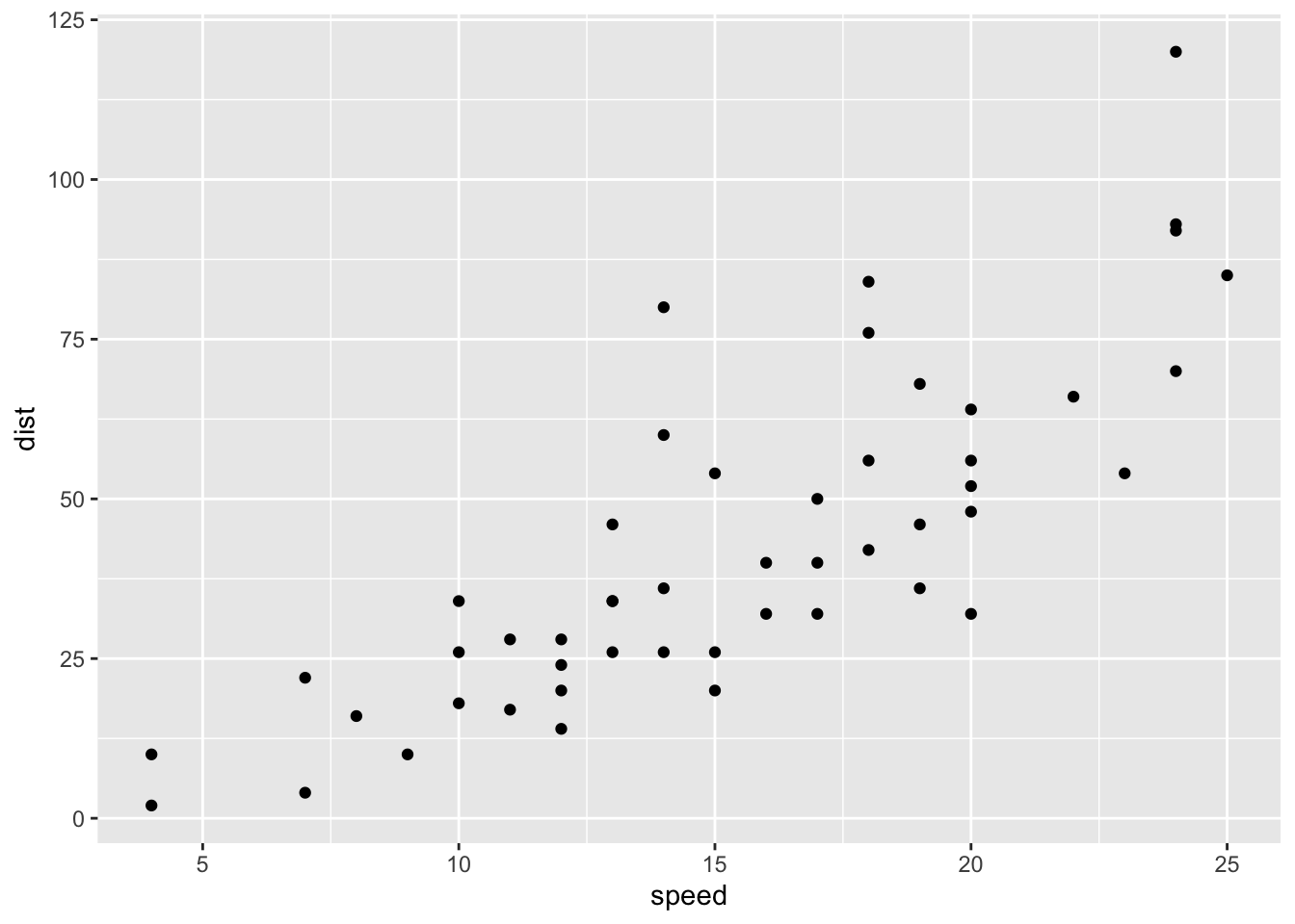
cor(cars)## speed dist
## speed 1.0000000 0.8068949
## dist 0.8068949 1.0000000The relationship appears linear and the correlation is sufficiently large (0.807), so we proceed with fitting a model.
mod.LinearCar = lm(dist~speed, data=cars)
summary(mod.LinearCar)
##
## Call:
## lm(formula = dist ~ speed, data = cars)
##
## Residuals:
## Min 1Q Median 3Q Max
## -29.069 -9.525 -2.272 9.215 43.201
##
## Coefficients:
## Estimate Std. Error t value Pr(>|t|)
## (Intercept) -17.5791 6.7584 -2.601 0.0123 *
## speed 3.9324 0.4155 9.464 1.49e-12 ***
## ---
## Signif. codes: 0 '***' 0.001 '**' 0.01 '*' 0.05 '.' 0.1 ' ' 1
##
## Residual standard error: 15.38 on 48 degrees of freedom
## Multiple R-squared: 0.6511, Adjusted R-squared: 0.6438
## F-statistic: 89.57 on 1 and 48 DF, p-value: 1.49e-12The coefficients, as well as their standard error and importance measure are given. We are also given the Residual standard error = \(\hat{\sigma}\) and Multiple R-squared which in this case (since it’s a simple linear model) is equal to the square of the correlation. The p-value associated with the variables test if we can drop the variable from the model, a large p-value indicates we can drop.
Additionally, we can view the ANOVA table of the model.
anova(mod.LinearCar)## Analysis of Variance Table
##
## Response: dist
## Df Sum Sq Mean Sq F value Pr(>F)
## speed 1 21186 21185.5 89.567 1.49e-12 ***
## Residuals 48 11354 236.5
## ---
## Signif. codes: 0 '***' 0.001 '**' 0.01 '*' 0.05 '.' 0.1 ' ' 1We see the model sum of squares (SSM) = \(\sum\limits_{i=1}^n(\hat{y}_i-\bar{y})^2\) (in this case SSM = 21186). We are also shown SSE = \(\sum\limits_{i=1}^n(y_i-\hat{y})^2\) (in this case SSE = 11354). We could calculate the sum of squares total as SST = SSM + SSE.
2.3.1 Making Predictions
If we wanted to predicted the average stopping distance for a car with speed = 15, we can construct a confidence interval with:
predict(mod.LinearCar, data.frame(speed=15), se.fit=T, interval='confidence',level=0.95)$fit## fit lwr upr
## 1 41.40704 37.02115 45.79292However, we could also predict the stopping distance for a particular car with speed = 15 by constructing a prediction interval:
predict(mod.LinearCar, data.frame(speed=15), se.fit=T, interval='prediction',level=0.95)$fit## fit lwr upr
## 1 41.40704 10.17482 72.63925The estimates in both cases are the same, however the confidence interval only considers variation from repeated experiments while a prediction interval considers this variance and the variation of an individual. For either case, the prediction will be more reliable near the center of the data.
Adding Line to Plot
We can easily add a linear model to our plot in the ggplot2 package. This also defaults to drawing a 95% confidence interval.
ggplot(cars, aes(speed, dist)) + geom_point() + geom_smooth(method='lm')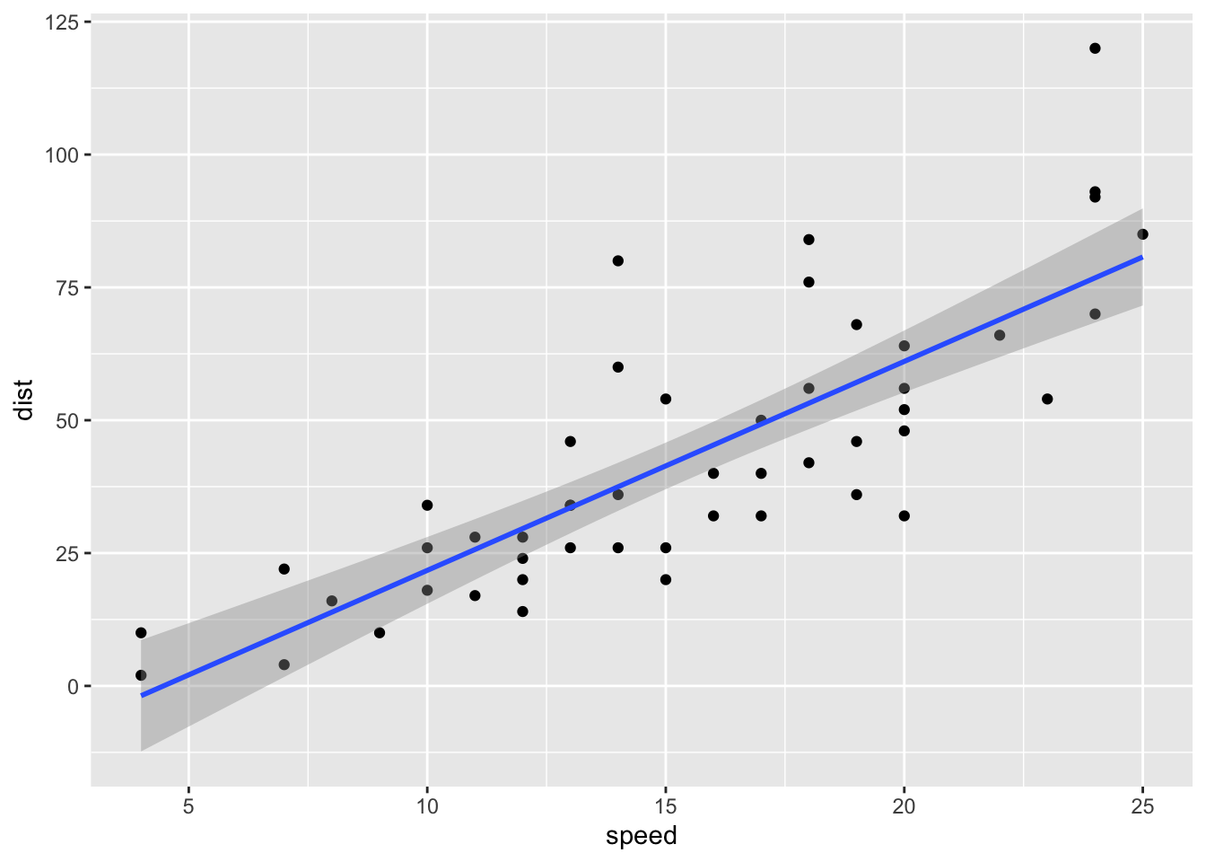
2.3.2 Checking Model Assumptions
Homoscedasticity
We assumed the spread of y’s is the same at any value of x. To check this,
plot(fitted.values(mod.LinearCar), residuals(mod.LinearCar), pch=16, xlab='Predicted Value', ylab='Residual')
abline(h=0, lty=2)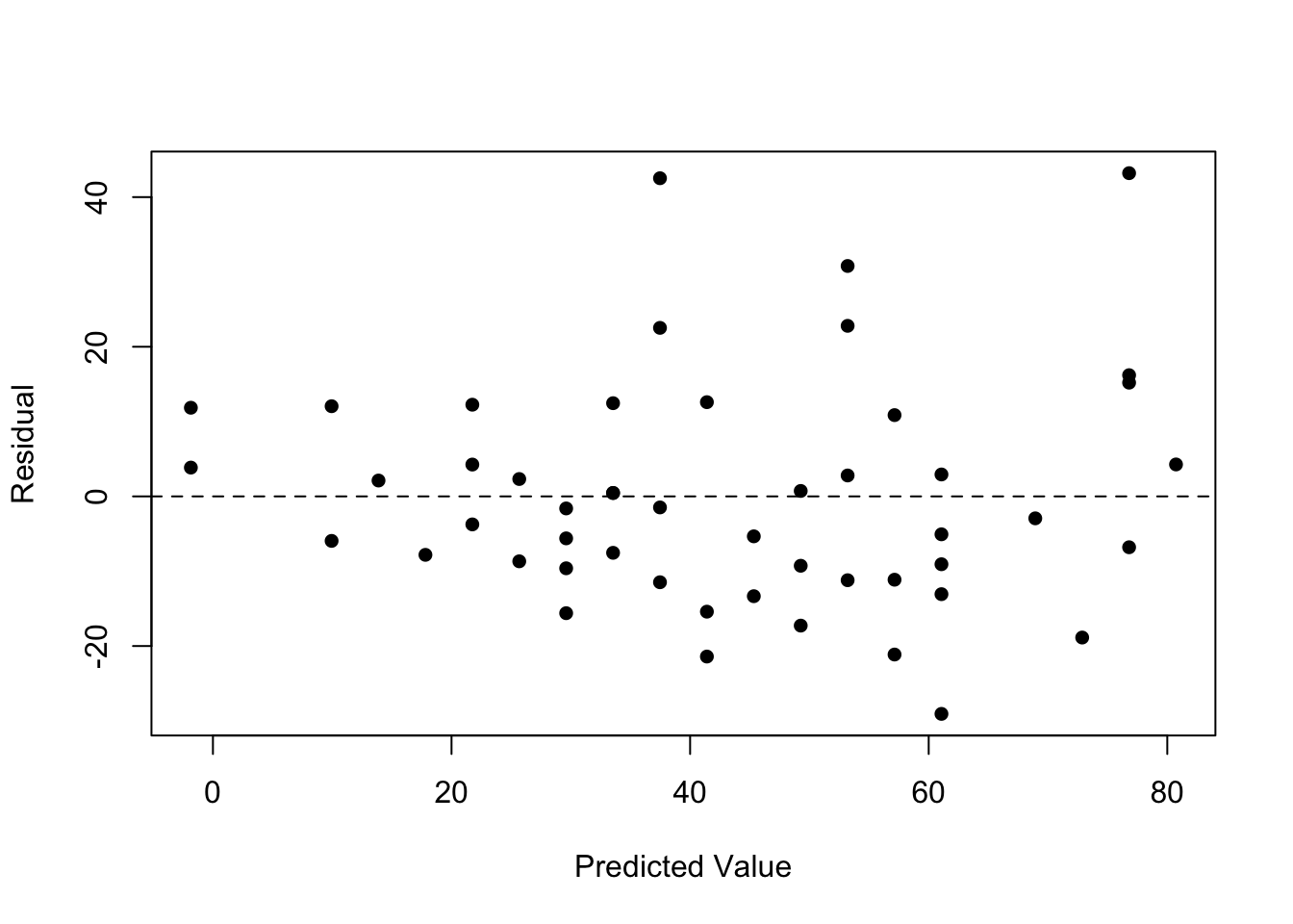
The residuals should be close to 0 and not have any pattern. If a pattern does exist (e.g. a funnel/triangle shape), we have evidence of non-homoscedasticity which could potentially be fixed by a data transformation.
Normality of Residuals
We also assumed our errors were normally distributed. To check this we will construct a QQ-plot:
qqnorm(residuals(mod.LinearCar), pch=16)
qqline(residuals(mod.LinearCar), col = "red", lwd = 2)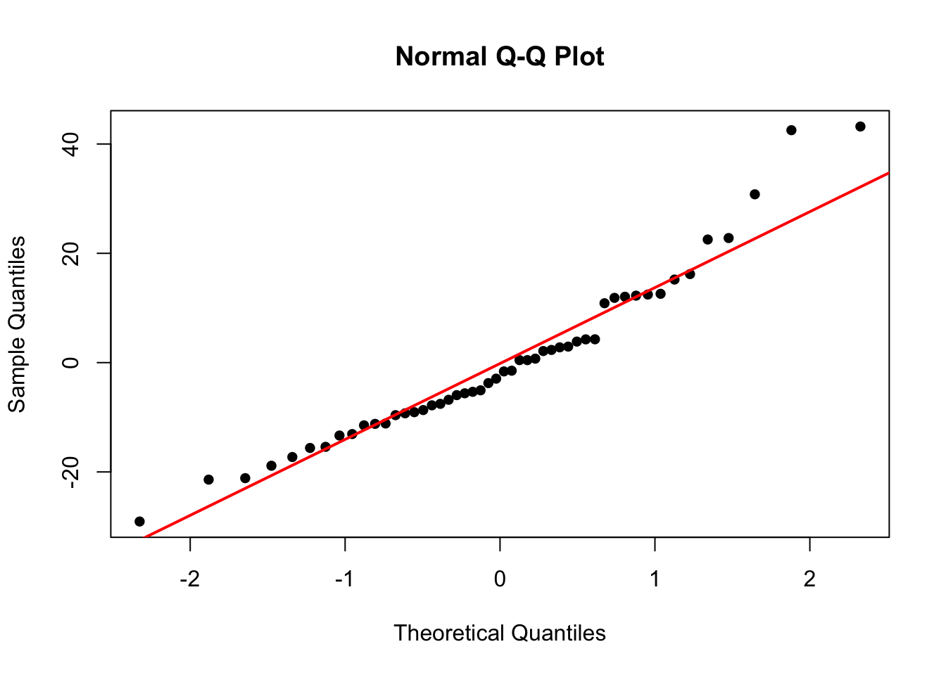
In this plot, Sample Quantiles refer to the actual value of the residuals, while Theoretical Quantiles are the z-scores of the residuals. If the residuals are normally distributed, the points should fall on/close to the reference line.
3 Multiple Linear Regression
Multiple linear regression is an extension of simple linear regression when there are several independent variables or functions of independent variables. For example, we could have two independent variables (\(y_i = \beta_0 + \beta_1 x_{i1} + \beta_2 x_{i2} + \varepsilon_i\)), a quadratic term (\(y_i = \beta_0 + \beta_1 x_{i1} + \beta_2 x_{i1}^2 + \varepsilon_i\)), or including an interaction term (\(y_i = \beta_0 + \beta_1 x_{i1} + \beta_2 x_{i2} + \beta_3 x_{i1}x_{i2} + \varepsilon_i\)). There can be non-linearity in x as long as the coefficients (\(\beta_i\)) maintain a linear relationship.
3.1 Multiple Linear Regression: Credit Example
We explore various models to predict credit card balance. This example was inspired by Springer’s book: An Introduction to Statistical Learning
We start with a model using all the available variables (except for ID). Note categorical variables are formatted as factors and are automatically converted to indicator/dummy variables.
library(ISLR)
head(Credit)
## ID Income Limit Rating Cards Age Education Gender Student Married Ethnicity Balance
## 1 1 14.891 3606 283 2 34 11 Male No Yes Caucasian 333
## 2 2 106.025 6645 483 3 82 15 Female Yes Yes Asian 903
## 3 3 104.593 7075 514 4 71 11 Male No No Asian 580
## 4 4 148.924 9504 681 3 36 11 Female No No Asian 964
## 5 5 55.882 4897 357 2 68 16 Male No Yes Caucasian 331
## 6 6 80.180 8047 569 4 77 10 Male No No Caucasian 1151mod.Full = lm(Balance ~ Cards + Limit + Rating + Age + Gender + Student + Income + Education + Married + Ethnicity, data=Credit)
summary(mod.Full)##
## Call:
## lm(formula = Balance ~ Cards + Limit + Rating + Age + Gender +
## Student + Income + Education + Married + Ethnicity, data = Credit)
##
## Residuals:
## Min 1Q Median 3Q Max
## -161.64 -77.70 -13.49 53.98 318.20
##
## Coefficients:
## Estimate Std. Error t value Pr(>|t|)
## (Intercept) -479.20787 35.77394 -13.395 < 2e-16 ***
## Cards 17.72448 4.34103 4.083 5.40e-05 ***
## Limit 0.19091 0.03278 5.824 1.21e-08 ***
## Rating 1.13653 0.49089 2.315 0.0211 *
## Age -0.61391 0.29399 -2.088 0.0374 *
## GenderFemale -10.65325 9.91400 -1.075 0.2832
## StudentYes 425.74736 16.72258 25.459 < 2e-16 ***
## Income -7.80310 0.23423 -33.314 < 2e-16 ***
## Education -1.09886 1.59795 -0.688 0.4921
## MarriedYes -8.53390 10.36287 -0.824 0.4107
## EthnicityAsian 16.80418 14.11906 1.190 0.2347
## EthnicityCaucasian 10.10703 12.20992 0.828 0.4083
## ---
## Signif. codes: 0 '***' 0.001 '**' 0.01 '*' 0.05 '.' 0.1 ' ' 1
##
## Residual standard error: 98.79 on 388 degrees of freedom
## Multiple R-squared: 0.9551, Adjusted R-squared: 0.9538
## F-statistic: 750.3 on 11 and 388 DF, p-value: < 2.2e-16From our output, we see Gender, Education, Married, Ethnicity are not significant, so we remove them from the model:
mod.Less = lm(Balance ~ Cards + Limit + Rating + Age + Student + Income, data=Credit)
summary(mod.Less)
##
## Call:
## lm(formula = Balance ~ Cards + Limit + Rating + Age + Student +
## Income, data = Credit)
##
## Residuals:
## Min 1Q Median 3Q Max
## -170.00 -77.85 -11.84 56.87 313.52
##
## Coefficients:
## Estimate Std. Error t value Pr(>|t|)
## (Intercept) -493.73419 24.82476 -19.889 < 2e-16 ***
## Cards 18.21190 4.31865 4.217 3.08e-05 ***
## Limit 0.19369 0.03238 5.981 4.98e-09 ***
## Rating 1.09119 0.48480 2.251 0.0250 *
## Age -0.62406 0.29182 -2.139 0.0331 *
## StudentYes 425.60994 16.50956 25.780 < 2e-16 ***
## Income -7.79508 0.23342 -33.395 < 2e-16 ***
## ---
## Signif. codes: 0 '***' 0.001 '**' 0.01 '*' 0.05 '.' 0.1 ' ' 1
##
## Residual standard error: 98.61 on 393 degrees of freedom
## Multiple R-squared: 0.9547, Adjusted R-squared: 0.954
## F-statistic: 1380 on 6 and 393 DF, p-value: < 2.2e-16Removing these variables results in a simpler model without sacrificing performance (\(R^2\) is similar).
3.1.1 Consider Multicollinearity
It is important our variables are not highly correlated with each other so that we have a design matrix of full rank and a unique solution to our minimization problem. To check this, we can compute the variance inflation factor for our variables, defined as \[VIF(X_m) = \frac{1}{1-R^2_m}\] where \(R^2_m\) is the coefficient of determination when \(X_m\) is regressed on all of the other predictors. We want \(VIF(X_m)\) to be close to 1, and a general rule is if it is larger than 5 or 10 there is a problem of multicollinearity.
For our simpler model, we calculate the VIF for each variable:
library(car)
vif(mod.Less)
## Cards Limit Rating Age Student Income
## 1.439007 229.238479 230.869514 1.039696 1.009064 2.776906The VIF for Limit and Rating is extremely high, indicating we should not include both of the variables in the model. We can calculate the correlation of these two variables and see it is close to 1.
cor(Credit$Limit, Credit$Rating)## [1] 0.9968797mod.LessNoRating = lm(Balance ~ Cards + Limit + Age + Student + Income, data=Credit)
summary(mod.LessNoRating)##
## Call:
## lm(formula = Balance ~ Cards + Limit + Age + Student + Income,
## data = Credit)
##
## Residuals:
## Min 1Q Median 3Q Max
## -187.05 -79.57 -12.59 56.06 322.56
##
## Coefficients:
## Estimate Std. Error t value Pr(>|t|)
## (Intercept) -4.673e+02 2.199e+01 -21.250 < 2e-16 ***
## Cards 2.355e+01 3.628e+00 6.492 2.55e-10 ***
## Limit 2.661e-01 3.535e-03 75.296 < 2e-16 ***
## Age -6.220e-01 2.933e-01 -2.120 0.0346 *
## StudentYes 4.284e+02 1.655e+01 25.886 < 2e-16 ***
## Income -7.760e+00 2.341e-01 -33.149 < 2e-16 ***
## ---
## Signif. codes: 0 '***' 0.001 '**' 0.01 '*' 0.05 '.' 0.1 ' ' 1
##
## Residual standard error: 99.12 on 394 degrees of freedom
## Multiple R-squared: 0.9541, Adjusted R-squared: 0.9535
## F-statistic: 1638 on 5 and 394 DF, p-value: < 2.2e-163.1.2 Checking Model Assumptions
Just like with the simple linear example, we need to verify our assumptions. We can plot our model to look for evidence of heteroscedasticity and non-normality:
plot(mod.LessNoRating, which=1)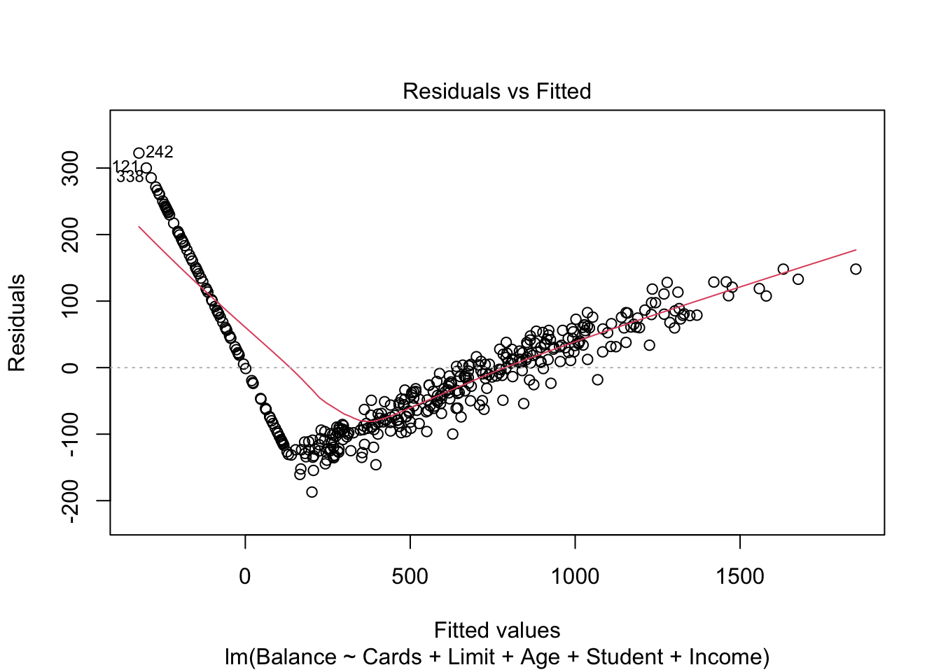
mod.LimitIncome = lm(Balance ~ Limit + Income, data=Credit)
plot(mod.LimitIncome, which=1)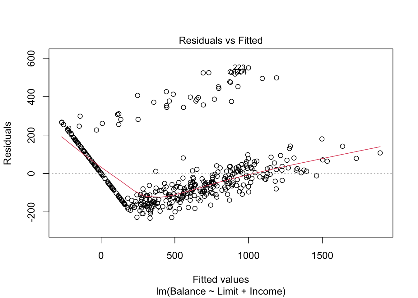
There are some concerns with our residuals which seem to be caused when both Limit and Income are included. The U-shape of the residuals indicate there may be something wrong with our model structure, and perhaps a quadratic term should be added. However, this U-shape only exists when both Limit and Income are included. If we remove one of these (removing Income resulted in a smaller drop in \(R^2\)), the concerns of heteroscedasticity are reduced.
mod.LessNoIncome = lm(Balance ~ Cards + Limit + Age + Student, data=Credit)
summary(mod.LessNoIncome)
##
## Call:
## lm(formula = Balance ~ Cards + Limit + Age + Student, data = Credit)
##
## Residuals:
## Min 1Q Median 3Q Max
## -657.27 -118.27 -2.56 137.66 449.07
##
## Coefficients:
## Estimate Std. Error t value Pr(>|t|)
## (Intercept) -3.074e+02 4.171e+01 -7.369 1.01e-12 ***
## Cards 2.950e+01 7.044e+00 4.188 3.48e-05 ***
## Limit 1.734e-01 4.201e-03 41.282 < 2e-16 ***
## Age -2.183e+00 5.628e-01 -3.878 0.000123 ***
## StudentYes 4.043e+02 3.214e+01 12.578 < 2e-16 ***
## ---
## Signif. codes: 0 '***' 0.001 '**' 0.01 '*' 0.05 '.' 0.1 ' ' 1
##
## Residual standard error: 192.7 on 395 degrees of freedom
## Multiple R-squared: 0.8261, Adjusted R-squared: 0.8243
## F-statistic: 469.1 on 4 and 395 DF, p-value: < 2.2e-16plot(mod.LessNoIncome, which=1)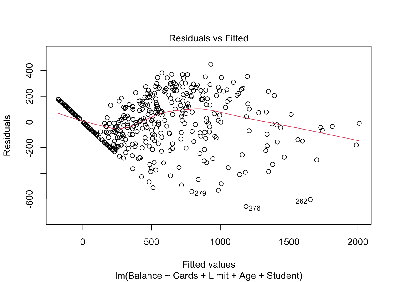
We can also check our residuals are normally distributed:
plot(mod.LessNoIncome, which=2)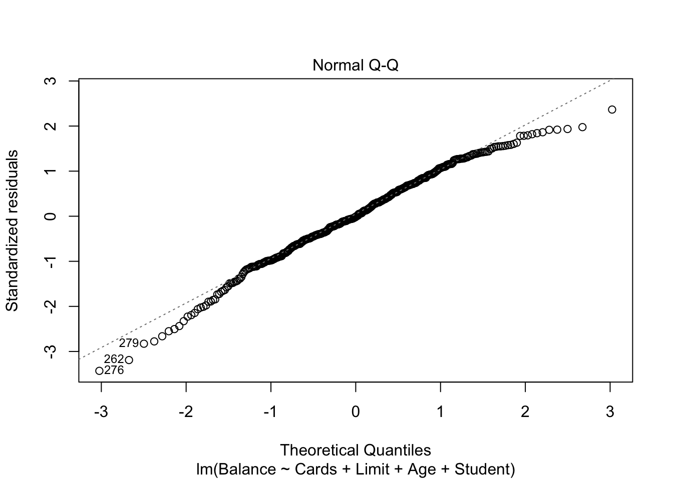
3.2 Adding an Interaction: Cars Example
So far we have assumed the effect of one predictor variable is independent of another, so all of our predictor variables are additive. However, it’s possible the variables are not independent and there is instead an interaction effect.
Using the mtcars data set, we try to predict miles per gallon (mpg) using horsepower (hp) and engine type (vs: v-shaped/straight). Without an interaction effect, our model produces two parallel lines, depending on the value of vs.
mod.NoInt = lm(mpg~hp+vs, mtcars)
mtcarsNoInt = cbind(mtcars, mpg.Fit = predict(mod.NoInt))
ggplot(mtcarsNoInt, aes(x = hp, y = mpg, colour = factor(vs))) + geom_point() + geom_line(aes(y=mpg.Fit))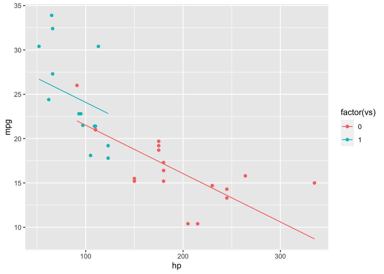
However, it is likely hp has a different effect on mpg depending on the engine type (vp). We add the interaction term to the model and see the lines are no longer parallel.
mod.Int = lm(mpg~hp+vs+hp*vs, mtcars)
mtcarsInt = cbind(mtcars, mpg.Fit = predict(mod.Int))
ggplot(mtcarsInt, aes(x = hp, y = mpg, colour = factor(vs))) + geom_point() + geom_line(aes(y=mpg.Fit))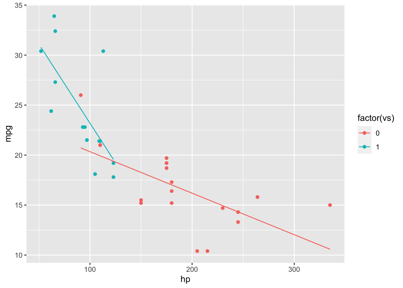
We can also examine the coefficients of our models:
summary(mod.NoInt)##
## Call:
## lm(formula = mpg ~ hp + vs, data = mtcars)
##
## Residuals:
## Min 1Q Median 3Q Max
## -5.7131 -2.3336 -0.1332 1.9055 7.9055
##
## Coefficients:
## Estimate Std. Error t value Pr(>|t|)
## (Intercept) 26.96300 2.89069 9.328 3.13e-10 ***
## hp -0.05453 0.01448 -3.766 0.000752 ***
## vs 2.57622 1.96966 1.308 0.201163
## ---
## Signif. codes: 0 '***' 0.001 '**' 0.01 '*' 0.05 '.' 0.1 ' ' 1
##
## Residual standard error: 3.818 on 29 degrees of freedom
## Multiple R-squared: 0.6246, Adjusted R-squared: 0.5987
## F-statistic: 24.12 on 2 and 29 DF, p-value: 6.768e-07summary(mod.Int)##
## Call:
## lm(formula = mpg ~ hp + vs + hp * vs, data = mtcars)
##
## Residuals:
## Min 1Q Median 3Q Max
## -5.5821 -1.7710 -0.3612 1.5969 9.2646
##
## Coefficients:
## Estimate Std. Error t value Pr(>|t|)
## (Intercept) 24.49637 2.73893 8.944 1.07e-09 ***
## hp -0.04153 0.01379 -3.011 0.00547 **
## vs 14.50418 4.58160 3.166 0.00371 **
## hp:vs -0.11657 0.04130 -2.822 0.00868 **
## ---
## Signif. codes: 0 '***' 0.001 '**' 0.01 '*' 0.05 '.' 0.1 ' ' 1
##
## Residual standard error: 3.428 on 28 degrees of freedom
## Multiple R-squared: 0.7077, Adjusted R-squared: 0.6764
## F-statistic: 22.6 on 3 and 28 DF, p-value: 1.227e-07The model with interaction has a larger \(R^2\) than the model without. It is interesting that vs is not significant in the first model but becomes significant when the interaction term is added.
The hierarchical principle tells us that within a model if the main effects variable (e.g. vs) is not significant but the interaction variable is (e.g. hp:vs), then we should still include the main effects variable. In our example, all the main effects variables were shown to be significant, but if one hadn’t and the interaction was significant, we should still include them.
A non-rigorous way to tell if an interaction variable is needed is to plot the data and visually fit a line by group. If the lines are parallel, no interaction is needed, but if they intersect (in this case), then an interaction should be considered.
3.3 Some Other Regression Topics
3.3.1 Model Selection
We have been using \(R^2\) to determine the percent of variation in the data is described by the model. We are also given the residual standard error, or root mean squared error (RMSE), in the model summary output.
Other model metrics
- Mallow’s \(C_p\): If this is small the model is competitive to the full model and preserves degrees of freedom
- Adjusted \(R^2\): Penalizes for too many predictors that don’t reduce unexplained variation
- \(PRESS_p\): Prediction Sum of Squares, if small then predicts point well
- BIC/AIC: Small if model is good fit and simple
Best subsets can be used to determine the best k models for a chosen number of variables.
Stepwise algorithms add/remove independent variables one at a time before converging to a best model. They can be either forward selection, backward elimination, or both. The algorithm may converge to different best models depending on the direction and initial model.
3.3.2 Leverage and Influence
- Leverage: Distance of an observation from the mean of the explanatory variables. The inclusion/exclusion of this observation has a large change on the fitted line
- Hat values - indicate potential for leverage
- Press residuals
- Studentized residuals
plot(mod.LessNoIncome, which=3)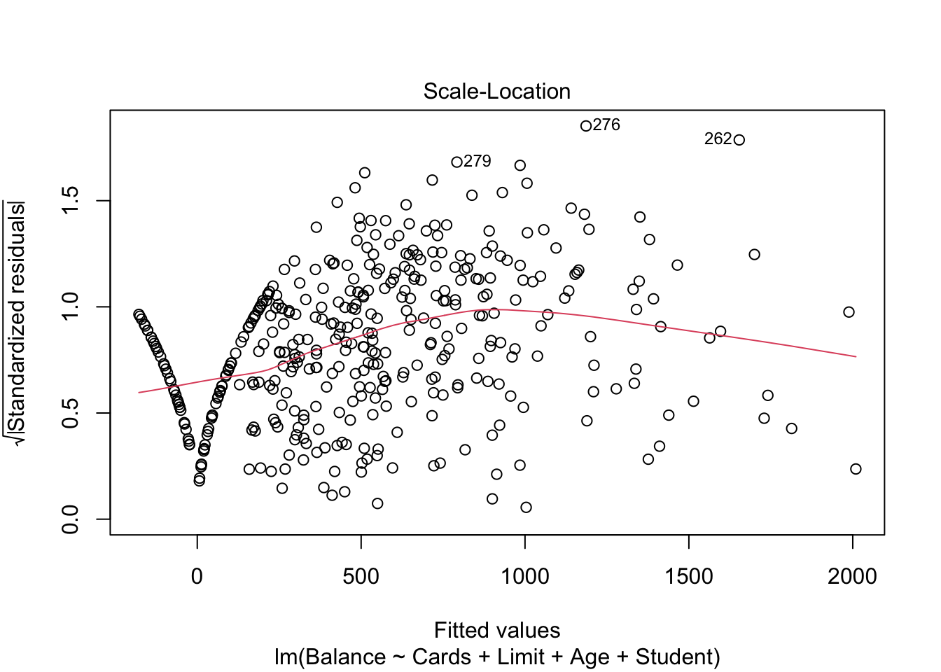
- Influence: Ability to change metrics of lines fit. For example, \(R^2 = 1-\frac{SSE}{SST}\), so adding a data point increases SST while it may keep SSE the same, artificially inflating \(R^2\).
- DFFITS - Difference in fits
- DfBetas - How much coefficients change when ith value is deleted
- Cook’s Distance - measures overall influence
plot(mod.LessNoIncome, which=4)
Alternative Definitions:
- Leverage: Extreme values, fitted line passes close to them
- Influence: Large effect on the model
- High influence typically implies high leverage
- High leverage doesn’t always imply high influence
set.seed(123)
df = data.frame(x = runif(100, min = -3, max = 3), y = runif(100, min = -1, max = 1))
ggplot(df, aes(x,y)) + geom_point() + geom_smooth(method = 'lm', se = F) +
  geom_text(aes(x=5, y=0.25), color = 'red', label = 'A') +
  geom_text(aes(x=4, y=4), color = 'red', label = 'B') +
  geom_text(aes(x=-0.1, y=-4), color = 'red', label = 'C') +
  xlim(-5,5) + ylim(-5,5)
## `geom_smooth()` using formula 'y ~ x'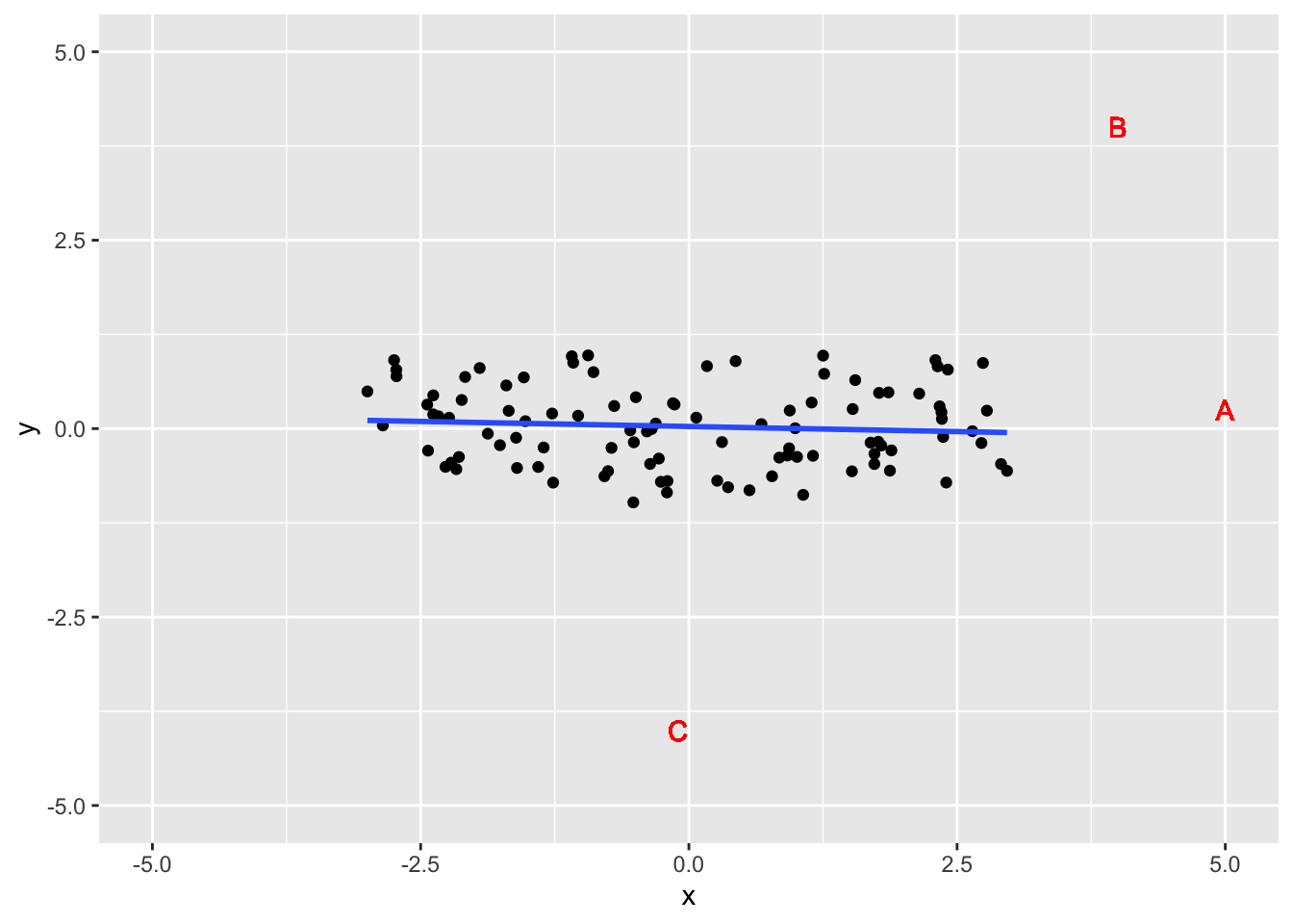
- Point A: High leverage, low influence
- Extreme x value, small change to line
- Point B: High leverage, high influence
- Extreme x value, large change to line
- Point C: Low leverage, low influence
- Not extreme x value, small change to line
4 Comparing Means
One-way analysis of variance (one-way ANOVA) allows us to compare means between two or more samples, where the repose variable is numeric and there is one explanatory variable (hence, one-way) that is generally categorical.
The one-factor ANOVA model is given by either the means model \[Y_{i,j} = \mu_i + \varepsilon_{i,j}\] or by the main effects model \[Y_{i,j} = \mu + \alpha_i + \varepsilon_{i,j}\] where \(Y_{i,j}\) is the jth observation at the ith treatment level, \(\mu\) is the grand mean, \(\mu_i\) is the mean of the observation for the ith treatment group, and \(\alpha_i\) is the ith treatment effect (deviation from the grand mean).
We have a balanced design if \(n_i\) is the same for all groups. If we think some treatment group has more variation we could use an unbalanced design.
We could also consider the two-factor ANOVA model which considers the influence of two explanatory variables. The (full) model is given by \[Y_{ijk} = \mu + \alpha_i + \beta_j + (\alpha\beta)_{ij} + \varepsilon_{ijk}\] where \(Y_{ijk}\) is the kth observation at the ith and jth treatment level, and \((\alpha\beta)_{ij}\) is the interaction effect.
ANOVA models perform an F-test to determine if all the group means are the same, or if at least one is statistically different. Various comparison and confidence interval methods allow us to determine which group is different.
The ANOVA model is a generalization of the simple linear regression model so it follows the same assumptions.
4.1 One-Factor ANOVA: Plant Growth Example
This example was inspired by One-way ANOVA
4.1.1 Fitting ANOVA Model
Our dataset include the weights of plants in a control group and two treatment groups. Notice the group column is formatted as a factor.
library(ggplot2)
growth = PlantGrowth
str(growth)
## 'data.frame': 30 obs. of 2 variables:
## $ weight: num 4.17 5.58 5.18 6.11 4.5 4.61 5.17 4.53 5.33 5.14 ...
## $ group : Factor w/ 3 levels "ctrl","trt1",..: 1 1 1 1 1 1 1 1 1 1 ...ggplot(growth, aes(group, weight)) + geom_boxplot()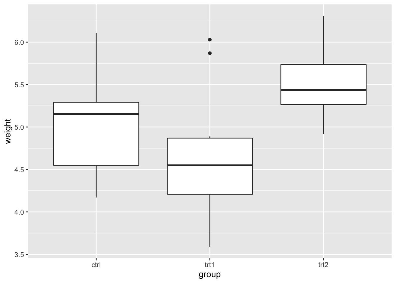
The boxplot indicates there may be a difference between treatments 1 and 2. We compute the one-way ANOVA test.
mod.aov = aov(weight~group, data = growth)
summary(mod.aov)
## Df Sum Sq Mean Sq F value Pr(>F)
## group 2 3.766 1.8832 4.846 0.0159 *
## Residuals 27 10.492 0.3886
## ---
## Signif. codes: 0 '***' 0.001 '**' 0.01 '*' 0.05 '.' 0.1 ' ' 1The p-value is less than 0.05 (our significance level), so there is evidence of a difference between some of the group means.
4.1.2 Checking Assumptions
Homoscedasticity
Like with the regression examples, we look for homogeneity of variances with a plot.
plot(mod.aov, which=1)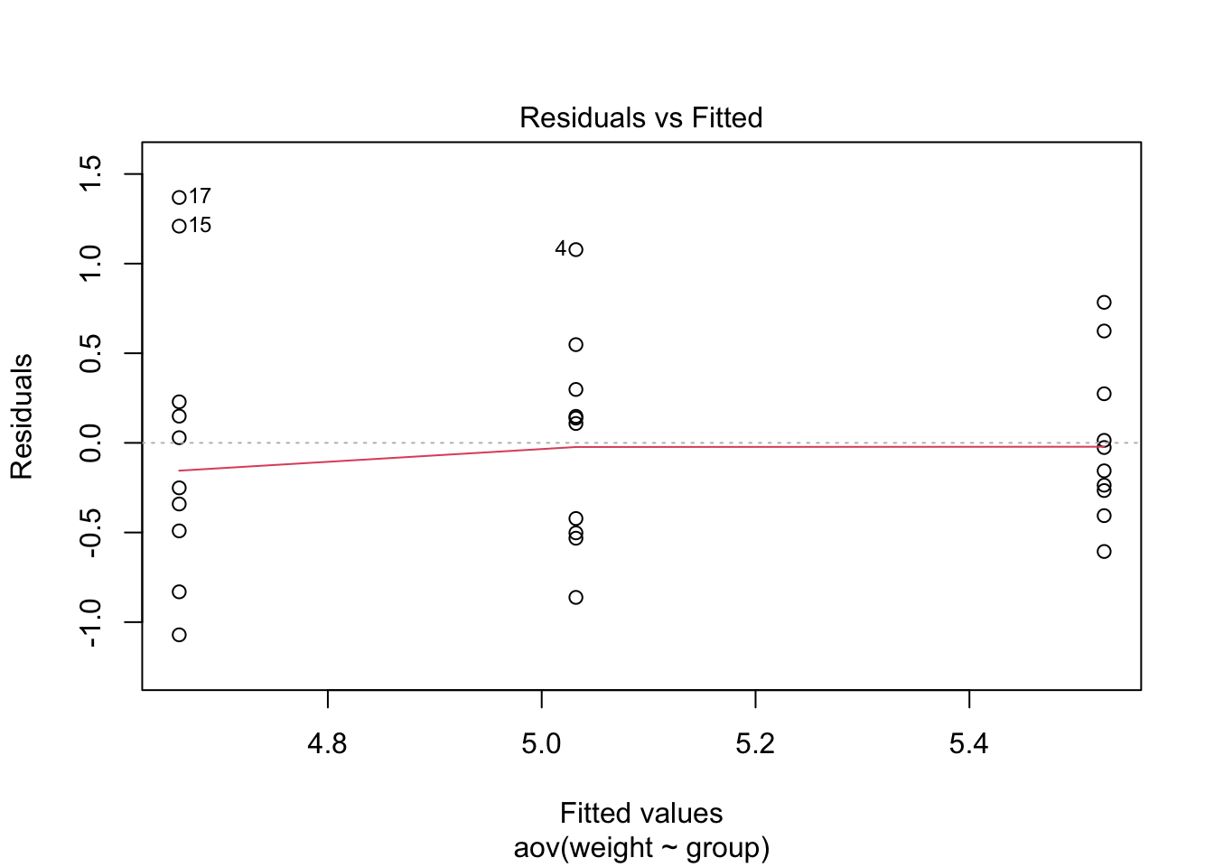
We could also use the Levene’s Test. For this, we fit an ANOVA model of the absolute residuals from our model against the groups. The F-statistic tests if there is a difference in the absolute mean residuals between the groups. If the test does detect a difference (small p-value), then there may be evidence of heteroscedasticity.
There is also a function in the car package to run the Levene’s Test.
summary(aov(abs(mod.aov$residuals)~group, data=growth))## Df Sum Sq Mean Sq F value Pr(>F)
## group 2 0.332 0.1662 1.237 0.306
## Residuals 27 3.628 0.1344library(car)
leveneTest(weight~group, data=growth)## Levene's Test for Homogeneity of Variance (center = median)
## Df F value Pr(>F)
## group 2 1.1192 0.3412
## 27Normality of Residuals
Again, we can check the normality of the residuals with a plot.
plot(mod.aov, which=2)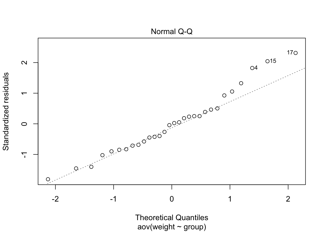
Note: observations 4, 15, and 17 may be outliers.
We can also use the Shapiro-Wilk test to determine if the residuals came from a normally distributed population.
shapiro.test(mod.aov$residuals)##
## Shapiro-Wilk normality test
##
## data: mod.aov$residuals
## W = 0.96607, p-value = 0.4379A large p-value means that we don’t reject the null hypothesis that our residuals are normally distributed.
4.1.3 Nonparametric Alternative
If the assumptions of the ANOVA are not met, we could use the Kruskal-Wallis test that does not assume a normal distribution of residuals. This test ranks all the data (ignoring group membership), computes a test statistic, then tests if all the groups have the same distribution.
The Dunn test can then be used to compute all pairwise comparisons (similar to Tukey’s pairwise comparisons method for ANOVA).
kruskal.test(weight~group, data=growth)##
## Kruskal-Wallis rank sum test
##
## data: weight by group
## Kruskal-Wallis chi-squared = 7.9882, df = 2, p-value = 0.01842library(FSA)
DT = dunnTest(weight~group, data=growth, method='bh')
DT## Comparison Z P.unadj P.adj
## 1 ctrl - trt1 1.117725 0.26368427 0.26368427
## 2 ctrl - trt2 -1.689290 0.09116394 0.13674592
## 3 trt1 - trt2 -2.807015 0.00500029 0.01500087library(rcompanion)
cldList(P.adj~Comparison, data = DT$res, threshold=0.05)## Group Letter MonoLetter
## 1 ctrl ab ab
## 2 trt1 a a
## 3 trt2 b bThe large p-value from the Kruskal-Wallis test tells us our groups come from different distributions. The Dunn test tells us there is a difference between treatment 1 and treatment 2.
4.2 Multiple Comparisons
The ANOVA test will determine if there is a difference between some of the groups, but won’t immediately tell us what groups are different. We can compute pairwise confidence intervals to determine which groups are different.
The general structure of a confidence interval is \(estimate \pm t_{dfe}*SE\), and various \(t_{dfe}\) and standard errors are possible.
4.2.1 T-Interval
Welch’s t-interval (Unpooled)
Welch’s t-interval is useful if we don’t think the population variances of the groups are equal. The standard error is given by \(\sqrt{\frac{s_1^2}{n_1}+\frac{s_2^2}{n_2}}\) where the standard deviations of the groups are kept separated.
In R, we calculate this by
control = growth$weight[growth$group=='ctrl']
treat1 = growth$weight[growth$group=='trt1']
treat2 = growth$weight[growth$group=='trt2']
t.test(control, treat1, var.equal=F, alternative = 'two.sided')$conf.int
## [1] -0.2875162 1.0295162
## attr(,"conf.level")
## [1] 0.95t.test(control, treat2, var.equal=F, alternative = 'two.sided')$conf.int## [1] -0.98287213 -0.00512787
## attr(,"conf.level")
## [1] 0.95t.test(treat1, treat2, var.equal=F, alternative = 'two.sided')$conf.int## [1] -1.4809144 -0.2490856
## attr(,"conf.level")
## [1] 0.95According to these intervals, there is a difference between control and treatment 2 and between treatment 1 and treatment 2.
Pooled t-interval
When we created the ANOVA model, we showed there was not a significant difference in variance between the groups, so we are able to pool the variance. In this case, our standard error is given by \(s_p\sqrt{\frac{1}{n_1} + \frac{1}{n_2}}\) where \(s_p\) is the pooled variance equal to \(\hat{\sigma}\).
In R, the confidence intervals are calculated similarly to the unpooled intervals, except now the variance is equal.
t.test(control, treat1, var.equal=T, alternative = 'two.sided')$conf.int## [1] -0.2833003 1.0253003
## attr(,"conf.level")
## [1] 0.95t.test(control, treat2, var.equal=T, alternative = 'two.sided')$conf.int## [1] -0.980338117 -0.007661883
## attr(,"conf.level")
## [1] 0.95t.test(treat1, treat2, var.equal=T, alternative = 'two.sided')$conf.int## [1] -1.4687336 -0.2612664
## attr(,"conf.level")
## [1] 0.95pairwise.t.test(growth$weight, growth$group)##
## Pairwise comparisons using t tests with pooled SD
##
## data: growth$weight and growth$group
##
## ctrl trt1
## trt1 0.194 -
## trt2 0.175 0.013
##
## P value adjustment method: holmThe intervals are slightly different than the unpooled intervals.
Using the standard t confidence interval to construct all the pair-wise confidence intervals is generally not recommended because it doesn’t consider the family-wise error rate, and results in artificially small intervals. This method should only be used if we’re interested in one pairwise contrast which was decided upon before looking at the data.
4.2.2 Family-wise error rate
Suppose our significance level (\(\alpha\)) is 0.05. If we construct one 95% confidence interval, the probability of making a type I error is 0.05.
The family-wise error rate is the probability of making at least one type I error in the family, defined as \[FWER \leq 1-(1-\alpha)^{I \choose 2} \] where \(\alpha\) is the significance level for an individual test and \({I \choose 2}\) is the number of pairwise comparisons given the total number of groups I.
If there are 3 groups, then there are 3 pairwise comparisons, and \(FWER \leq 0.1426\). If there are 5 groups, then there are 10 pairwise comparisons, and \(FWER \leq 0.4013\), etc.
As the number of groups grows, the upper bound for FWER also grows. So, as increase groups, the probability of a type I error becomes very high. Some ways to control this include the Bonferroni correction, Tukey’s procedure, and Scheffe’s method
4.2.3 Bonferonni Correction
The Bonferroni correction constructs each individual confidence interval at a higher level to result in a higher family-wise confidence level. The individual confidence level is \(\frac{\alpha}{m}\) where m is the total number of intervals to construct (often \(m = {I \choose 2}\)). So, each confidence interval will have a \(1-\frac{\alpha}{m}\) level of confidence. The Bonferonni correction is typically only recommended for 3 or 4 groups.
For our example, we had 3 groups so each pairwise confidence interval will be constructed at the 98.3% confidence level.
library(DescTools)
PostHocTest(mod.aov, method='bonferroni')
##
## Posthoc multiple comparisons of means : Bonferroni
## 95% family-wise confidence level
##
## $group
## diff lwr.ci upr.ci pval
## trt1-ctrl -0.371 -1.0825786 0.3405786 0.5832
## trt2-ctrl 0.494 -0.2175786 1.2055786 0.2630
## trt2-trt1 0.865 0.1534214 1.5765786 0.0134 *
##
## ---
## Signif. codes: 0 '***' 0.001 '**' 0.01 '*' 0.05 '.' 0.1 ' ' 1These intervals tell us only the difference between treatment 1 and treatment 2 are statically significant.
4.2.4 Tukey Procedure
The Tukey method uses the studentized range distribution to create simultaneous comparisons for all pairwise comparisons.
We can compute all the pairwise Tukey intervals in R.
TukeyHSD(mod.aov)## Tukey multiple comparisons of means
## 95% family-wise confidence level
##
## Fit: aov(formula = weight ~ group, data = growth)
##
## $group
## diff lwr upr p adj
## trt1-ctrl -0.371 -1.0622161 0.3202161 0.3908711
## trt2-ctrl 0.494 -0.1972161 1.1852161 0.1979960
## trt2-trt1 0.865 0.1737839 1.5562161 0.0120064We can also visualize the intervals
plot(TukeyHSD(mod.aov))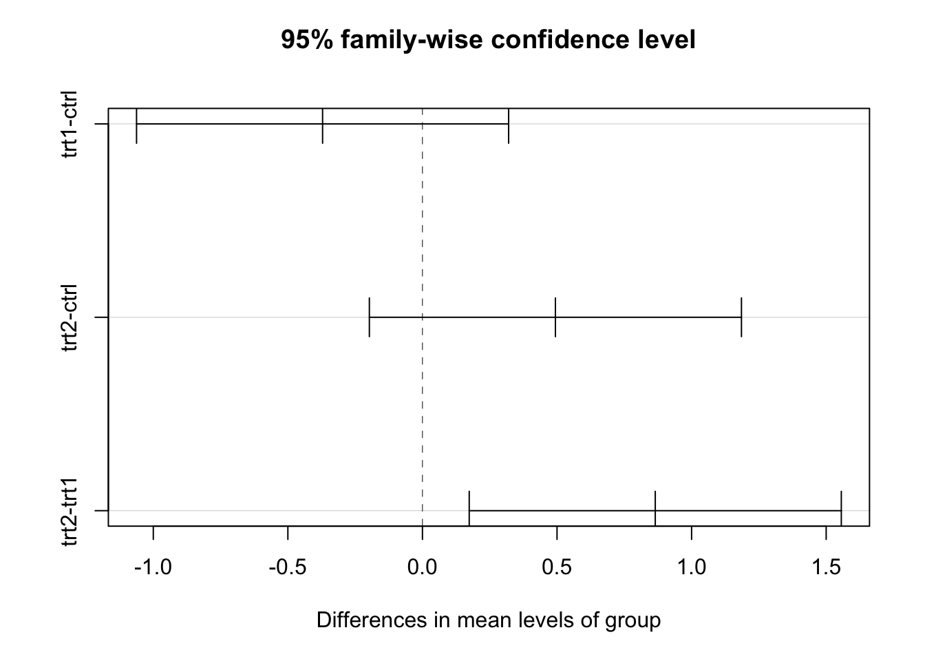
The conclusion is the same as with the Bonferonni correction (treatment 1 and 2 are different), however the Tukey method works well for many groups.
4.2.5 Scheffe’s Method
Scheffe’s method is useful for any type of contrast, not just pairwise differences. A confidence interval for contrast \(\Psi = \sum\limits_{i=1}^Ic_iy_i\) is given by \[\sum\limits_{i=1}^Ic_i\hat{y}_i \pm \sqrt{(I-1)F_{I-1,n-1}^\alpha}*\hat{\sigma}\sqrt{\sum\limits_{i=1}^I\frac{c_i^2}{n_i}}\] For example, suppose we want a confidence interval for \(y_{control} - \frac{y_{treat1} + y_{treat2}}{2}\) which compares control to the average of the treatments.
ScheffeTest(mod.aov, contrasts = matrix(c(1,-0.5,-0.5,
                                          -0.5,1,-0.5,
                                          -0.5,-0.5,1),ncol=3))
##
## Posthoc multiple comparisons of means: Scheffe Test
## 95% family-wise confidence level
##
## $group
## diff lwr.ci upr.ci pval
## ctrl-trt1,trt2 -0.0615 -0.6868163 0.563816298 0.9681
## trt1-ctrl,trt2 -0.6180 -1.2433163 0.007316298 0.0532 .
## trt2-ctrl,trt1 0.6795 0.0541837 1.304816298 0.0310 *
##
## ---
## Signif. codes: 0 '***' 0.001 '**' 0.01 '*' 0.05 '.' 0.1 ' ' 1The first row of the output table shows there is not a significant difference between the control group and the average of the treatment groups.
The second row shows there may be a difference between treatment 1 and the average of control and treatment 2.
The third row shows there is likely a difference between treatment 2 and the average between control and treatment 1.
4.3 Two-Factor ANOVA: Strength Example
Data for this example were modified from an assignment in one of my graduate courses. Our goal is to determine if substrate or bonding material are useful in predicting strength.
4.3.1 Analyzing the Data
library(tidyverse)
strength = c(1.51,1.96,1.83,1.98, 2.62,2.82,2.69,2.93, 2.96,2.82,3.11,3.11, 3.67,3.4,3.25,2.9,
             1.63,1.8,1.92,1.71, 3.12,2.94,3.23,2.99, 2.91,2.93,3.01,2.93, 3.48,3.51,3.24,3.45,
             3.04,3.16,3.09,3.5, 1.19,2.11,1.78,2.25, 3.04,2.91,2.48,2.83, 3.47,3.42,3.31,3.76)
substrate = c(rep("A",16), rep("B", 16), rep("C", 16))
material = c(rep( c(rep("E1",4), rep("E2",4), rep("S1",4), rep("S2",4)),3))
bonds = data.frame(substrate, material, strength) %>% mutate_if(is.character, factor)
plot(strength~substrate,bonds) 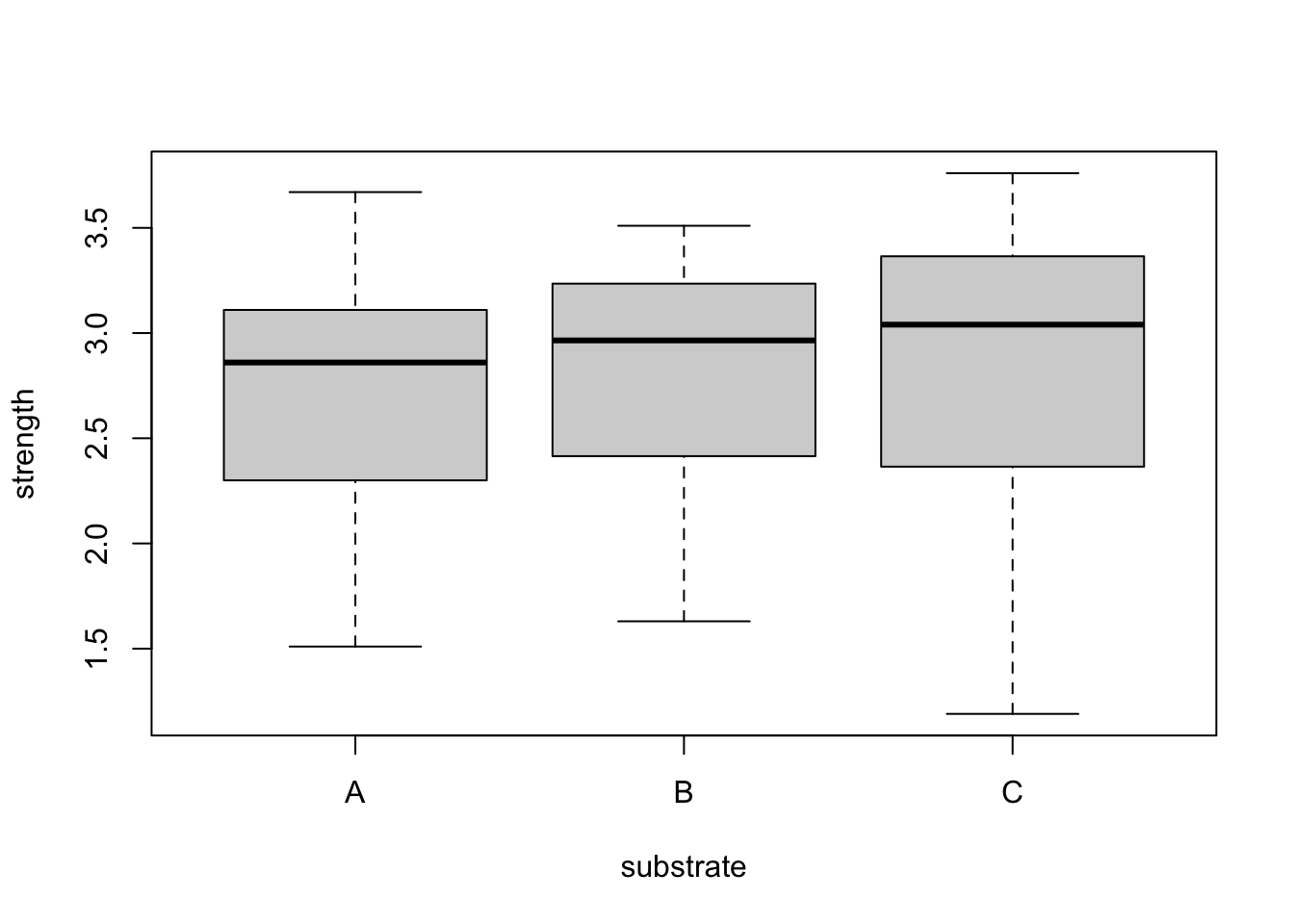
plot(strength~material,bonds)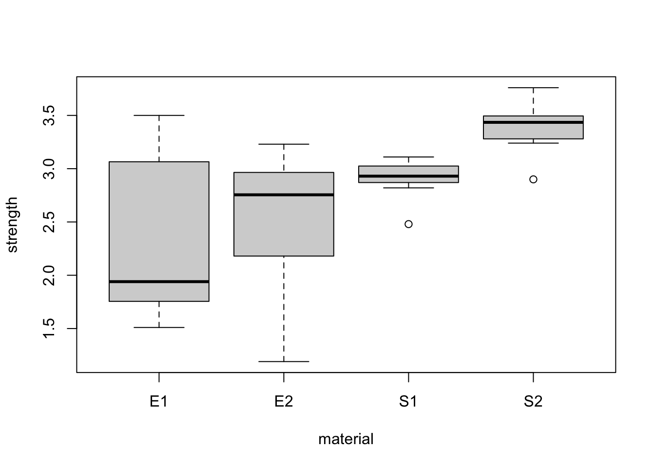
It appears material has a greater impact on strength than substrate. We also consider the interaction between substrate and material.
interaction.plot(bonds$substrate, bonds$material, bonds$strength, xlab="Substrate", ylab="Mean Strength")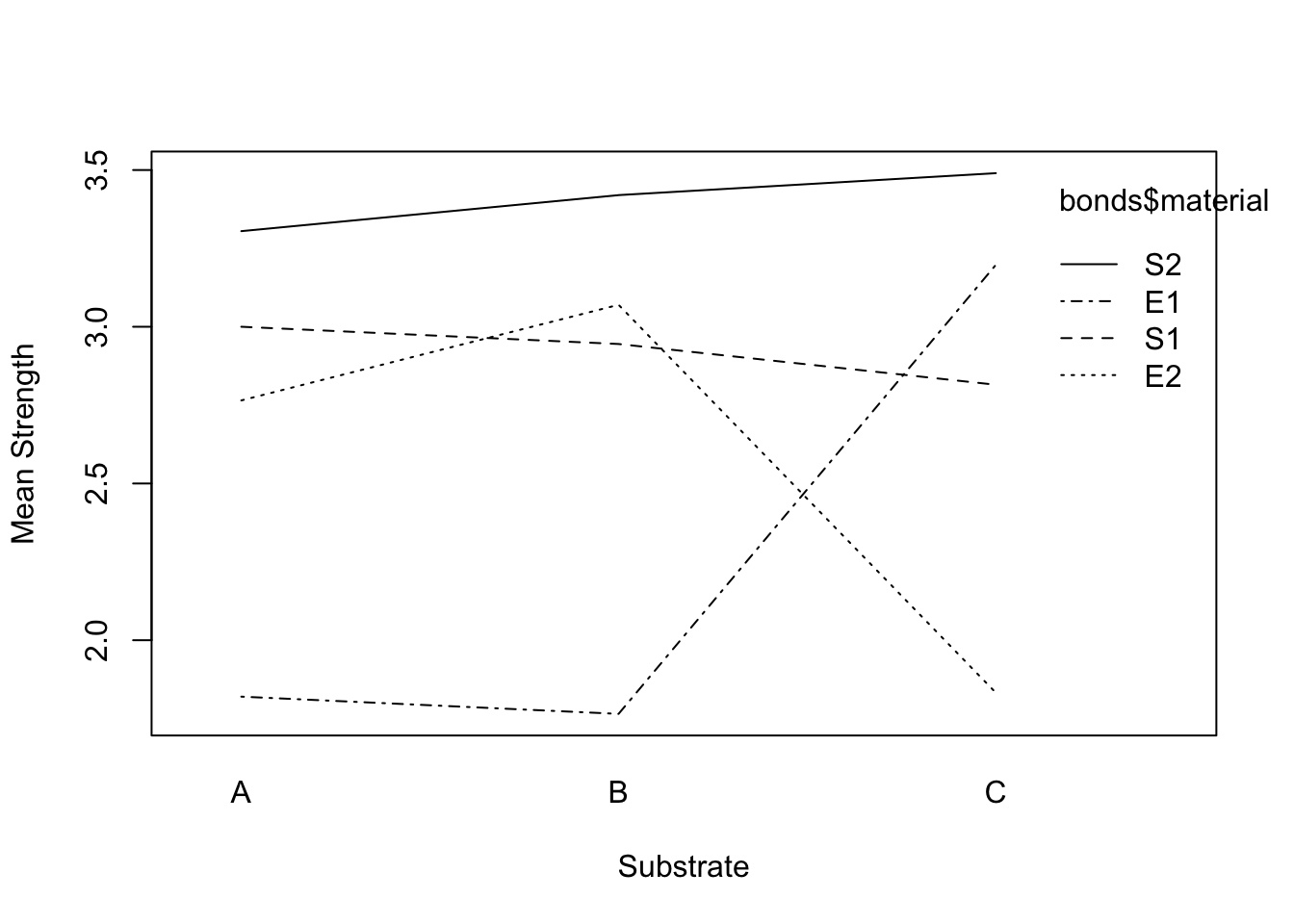
interaction.plot(bonds$material, bonds$substrate, bonds$strength, xlab="Material", ylab="Mean Strength")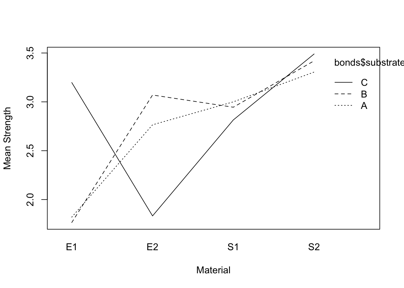
The lines are not parallel indicating interaction may be significant.
4.3.2 ANOVA Model
We fit the full 2-way ANOVA model. Any of the fitting methods can be used and produce the same results.
mod.aov2Full = lm(strength ~ material + substrate + material*substrate, data = bonds)
#mod.aov2Full = lm(strength~material*substrate, data=bonds)
#mod.aov2Full = aov(strength~material*substrate, data=bonds)
#mod.aov2Full = aov(strength ~ material + substrate + material*substrate, data = bonds)
#mod.aov2Full = aov(strength ~ material + substrate + material:substrate, data = bonds)
summary(mod.aov2Full)
##
## Call:
## lm(formula = strength ~ material + substrate + material * substrate,
## data = bonds)
##
## Residuals:
## Min 1Q Median 3Q Max
## -0.64250 -0.08687 -0.00250 0.11000 0.41750
##
## Coefficients:
## Estimate Std. Error t value Pr(>|t|)
## (Intercept) 1.820e+00 1.116e-01 16.308 < 2e-16 ***
## materialE2 9.450e-01 1.578e-01 5.988 7.22e-07 ***
## materialS1 1.180e+00 1.578e-01 7.477 7.86e-09 ***
## materialS2 1.485e+00 1.578e-01 9.409 3.08e-11 ***
## substrateB -5.500e-02 1.578e-01 -0.348 0.730
## substrateC 1.377e+00 1.578e-01 8.728 2.06e-10 ***
## materialE2:substrateB 3.600e-01 2.232e-01 1.613 0.115
## materialS1:substrateB 3.150e-16 2.232e-01 0.000 1.000
## materialS2:substrateB 1.700e-01 2.232e-01 0.762 0.451
## materialE2:substrateC -2.310e+00 2.232e-01 -10.349 2.46e-12 ***
## materialS1:substrateC -1.562e+00 2.232e-01 -7.000 3.28e-08 ***
## materialS2:substrateC -1.192e+00 2.232e-01 -5.343 5.25e-06 ***
## ---
## Signif. codes: 0 '***' 0.001 '**' 0.01 '*' 0.05 '.' 0.1 ' ' 1
##
## Residual standard error: 0.2232 on 36 degrees of freedom
## Multiple R-squared: 0.907, Adjusted R-squared: 0.8786
## F-statistic: 31.93 on 11 and 36 DF, p-value: 2.848e-15anova(mod.aov2Full)## Analysis of Variance Table
##
## Response: strength
## Df Sum Sq Mean Sq F value Pr(>F)
## material 3 8.7587 2.91957 58.605 6.268e-14 ***
## substrate 2 0.1041 0.05206 1.045 0.3621
## material:substrate 6 8.6333 1.43889 28.883 2.312e-12 ***
## Residuals 36 1.7934 0.04982
## ---
## Signif. codes: 0 '***' 0.001 '**' 0.01 '*' 0.05 '.' 0.1 ' ' 1The ANOVA output shows substrate may not be significant to the model (it also didn’t appear to be significant in the initial boxplot). However, if we remove substrate we must also remove the interaction term (to maintain a hierarchical model). We test if the coefficients for substrate and interaction terms are 0.
We first compute the F-statistic: \[F = \frac{[SSE_{Reduced} - SSE_{Full}]/[dfe_{Reduced}-dfe_{Full}]}{MSE_{Full}} = \frac{(0.1041+8.6333)/(2+6)}{0.04982}\] Then, we compare this F-statistic to the F distribution with 8 and 36 degrees of freedom to obtain the p-value.
Fstat = ((0.1041 + 8.6333)/(2+6)) / 0.04982
pvalue = pf(Fstat, 8,36,lower.tail = FALSE)
pvalue
## [1] 1.140389e-11The small p-value means we reject the null hypothesis and conclude we cannot drop the substrate and interaction terms.
4.3.3 Checking Assumptions
Homoscedasticity
We check the assumption of homoscedasticity with a plot (we could also use Levene’s test)
plot(mod.aov2Full, which=1)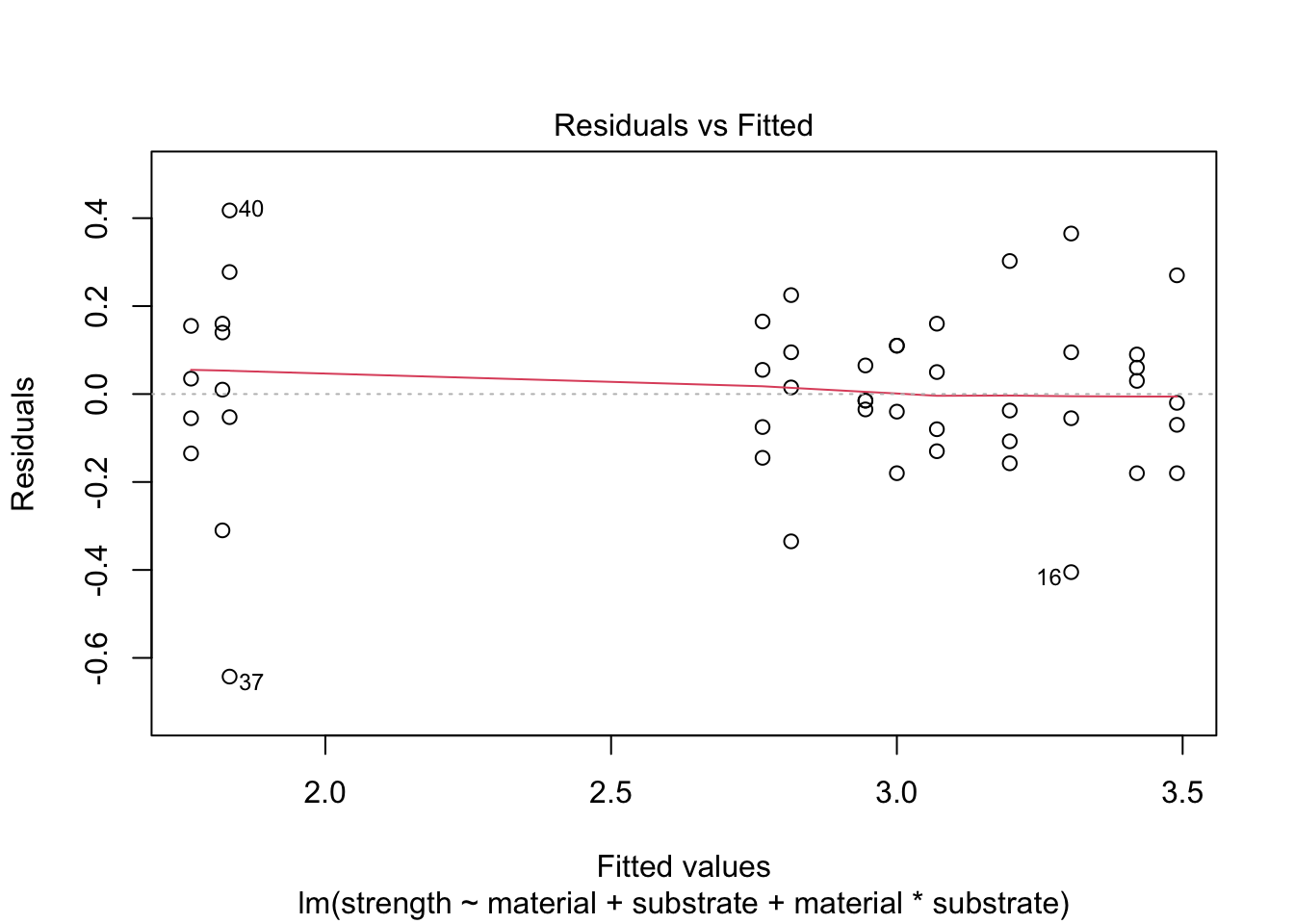
There may be some outliers but not overwhelming evidence of heteroscedasticity.
Normality of Residuals
We also check the distribution of the residuals with a plot (we could use the Shapiro-Wilk test).
plot(mod.aov2Full, which=2)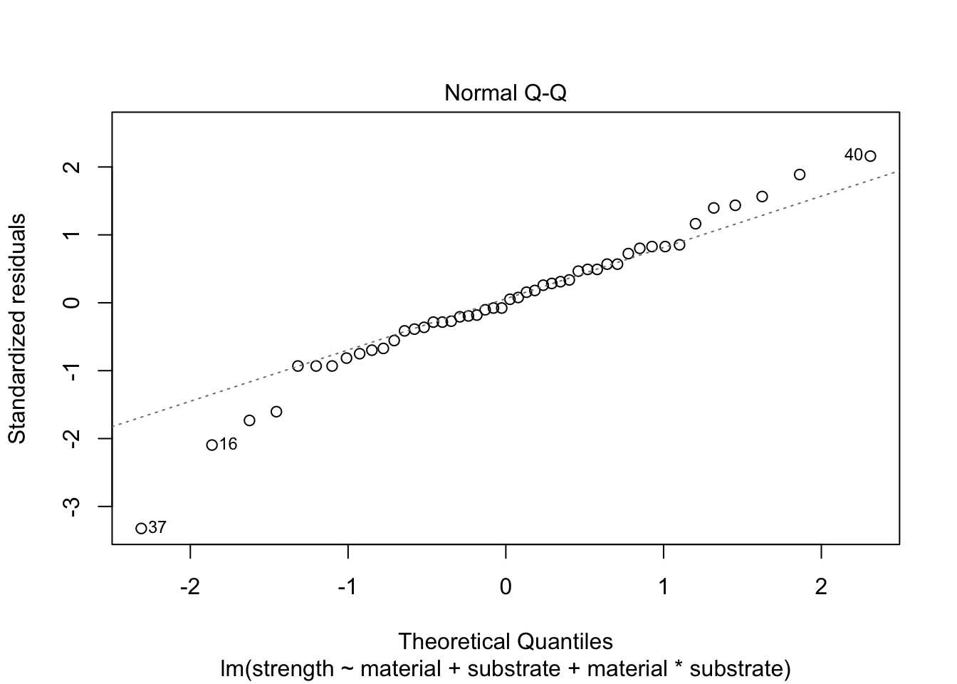
4.3.4 Making Predictions
If we want to determine which combination(s) of material and substrate produce the greatest strength, we could start by computing all bonding material pairwise confidence intervals.
mod.aov2Full = aov(strength ~ material + substrate + material:substrate, data = bonds)
TukeyHSD(mod.aov2Full,which = 'material', conf.level = 0.95) #TukeyHSD requires an ANOVA object
## Tukey multiple comparisons of means
## 95% family-wise confidence level
##
## Fit: aov(formula = strength ~ material + substrate + material:substrate, data = bonds)
##
## $material
## diff lwr upr p adj
## E2-E1 0.2950000 0.04959085 0.5404091 0.0132102
## S1-E1 0.6591667 0.41375752 0.9045758 0.0000001
## S2-E1 1.1441667 0.89875752 1.3895758 0.0000000
## S1-E2 0.3641667 0.11875752 0.6095758 0.0016623
## S2-E2 0.8491667 0.60375752 1.0945758 0.0000000
## S2-S1 0.4850000 0.23959085 0.7304091 0.0000321This output tells us there is a significant difference between all bonding materials.
We could also plot the mean of each combination with their standard errors. Note, since we are using the full model, the predictions for each of the 12 treatments combinations are equal to each of the cell means.
meanData = bonds %>% group_by(substrate, material) %>% summarise(strength = mean(strength))## `summarise()` has grouped output by 'substrate'. You can override using the `.groups` argument.sigma = sqrt(.04982)
se = sigma/sqrt(4)
pd = position_dodge(0.1)
ggplot(meanData, aes(x=substrate, y=strength, colour=material, group=material)) +
geom_errorbar(aes(ymin=strength-se, ymax=strength+se), colour="black", width=.25, position=pd) +
geom_line(position=pd) +
geom_point(position=pd, size=4, shape=21, fill="white")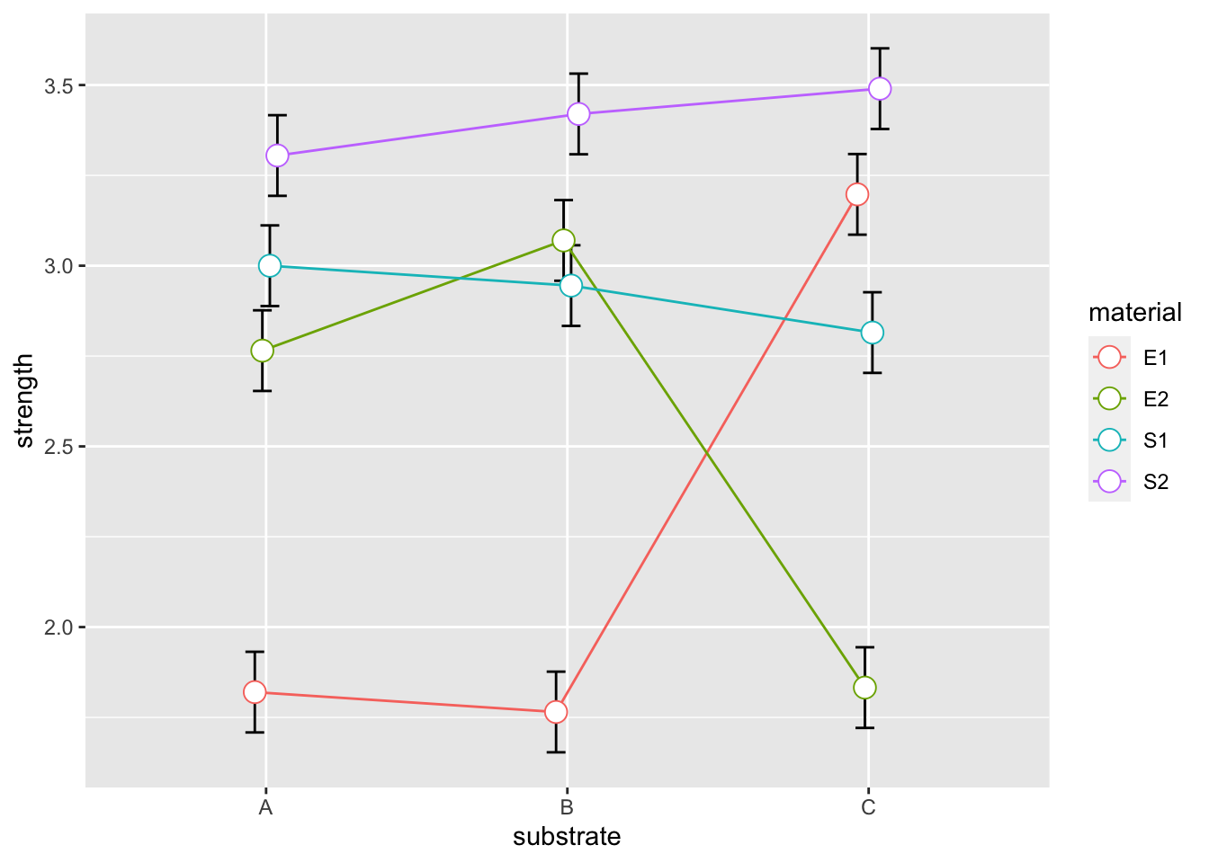
To obtain the greatest strength we should use material S2 with any substrate.
5 Binomial Regression
Goal: predict odds of seeing an event given a vector of regression variables. GLMs model relationship between E(y) and linear combination of vector X.
Probability mass function of binomially distributed y: \[Pr(y_i = k | X = x_i) = {m \choose k} \pi_i^k (1-\pi_i)^{m-k}\]
Probability of success \(\pi_i\) for some \(X = x_i\) given by some function g(.) \[ \pi_i = g(x_i)\]
Relationship between E(y|X) and X expressed by link function: \[ g(E(y = y_i|X = x_i)) = \sum_{j=0}^p \beta_j x_{ij} \] where X is (nXp), n = number of rows, p = regression variables, \(\beta\) is (pX1)
When y is binomially distributed, fix relation between conditional expectation of the probability \(\pi\) of a single Bernoulli trial on a particular value of \(X = x_i\). GLM for binomial regression model: \[ g(E(\pi = \pi_i|X = x_i)) = g(\pi_i|x_i) = \sum_{j=0}^p \beta_i x_{ij} \] with various possible link functions.
5.1 Link Functions
*Logistic (logit, log-odds): \(g(\pi_i) = ln \left( \frac{\pi_i}{1-\pi_i} \right)\) -> \(\pi_i = \frac{e^{\beta x_i}}{1+e^{\beta x_i}}\)
*Probit: \(g(\pi_i) = \Phi^{-1}(\pi_i)\)
*Log-log: \(g(\pi_i) = ln(-ln(pi_i))\)
*Complementary log-log: \(g(\pi_i) = ln(-ln(1-\pi_i))\)