Model Validation

1 R-squared

\[R^2 = \frac{\sum(y_i - \bar{y})^2 - \sum(y_i - \hat{y_i})^2}{\sum(y_i - \bar{y})^2}\] Perfect model: \(\hat{y_i} = y_i\) so \(R^2 = 1\)

2 Gini

Ratio of how close model is to perfect model and how far it is from a random model. Gini = 1 → perfect model, Gini = 0 → random model

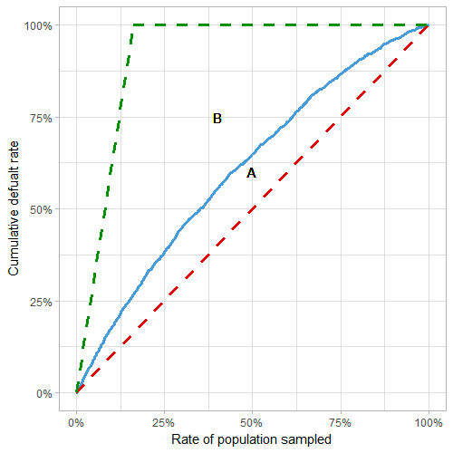
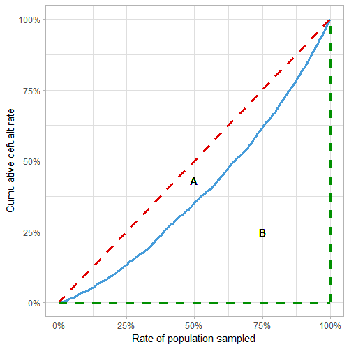
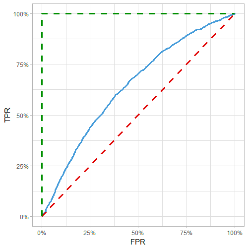
This article derives Gini using three methods: from the CAP curve, from the Lorenz curve, and from the ROC curve.

• In all cases, order data by prediction, plot cumulative response vs cumulative proportion of sample

• Red line: random model, blue line: actual model, green line: perfect model

  • Gini = A/(A+B) = 2*AUC - 1

From CAP curve:

From Lorenz curve:

From ROC curve:

3 Lift Chart

3.1 Single Lift

• Order data by prediction/weight, group into bins (e.g. deciles) with equal weight (e.g. earned car years)

• Within each bin, get average predicted and actual value

3.2 Double Lift

For comparing 2 predictions to actual

• Order data by prediction_1/prediction_2, group into bins

• Within each bin, get averaged prediction_1, prediction_2, and actual value

4 Binomial Deviance

Deviance = \(2 \sum o_i log \left( \frac{o_i}{e_i} \right)\) where \(o_i\) denotes observed, \(e_i\) denotes expected, and the sum is over both successes and failures for each i

• Gives measure of deviance of fitted glm with respect to perfect model (aka saturated model, a model that perfectly fits the data)

• Alternate definitions: Deviance = \(-2 \left[ l(\hat{\beta}) - l_s \right]\) where the log-likelihood of the fitted model \(l(\hat{\beta})\) is always smaller than the saturated model

  • For a linear model, Deviance = \(RSS(\hat{\beta})\) = SSE

  • Deviance is always greater than or equal to 0, if 0 then the fit is perfect

• Generally compared to null deviance \(D_0 = -2 \left[ l(\hat{\beta}_0) - l_s \right]\) which compares a model without predictors (intercept only) to the perfect model

  • For a linear model, \(D_0\) = SST

• To quantify the percent of deviance explained (ratio indicating how close the fit is to being perfect) use \(R^2 = 1- \frac{D}{D_0}\)

  • For a linear model, \(R^2 = 1-\frac{SSE}{SST}\)

  • Also known as McFadden’s R²= \(1 - \frac{log(L_{full})}{log(L_{intercept})}\) where L_full is the likelihood value from the fitted model.

    • The likelihood contribution of each observation is between 0 and 1, so the log likelihood is always negative

    • If the model has no predictive ability → likelihood of model similar to likelihood of intercept → R² close to 0

    • If model explains almost everything → likelihood value for each observation close to 1 → log(1) = 0 → R² close to 1

• In R, deviance is returned in summary as “Residual deviance” and “Null deviance”

• To calculate log likelihood of fitted model: \(\sum \left( log(\hat{y}_i)*y_i + log(1-\hat{y}_i)*(1-y_i) \right)\) where \(\hat{y_i}\) is the fitted probability and \(y_i\) is the actual response value

  • For the null model: use \(\hat{y} = mean(y)\) using the y values from the training data

5 Metrics from Confusion Matrix

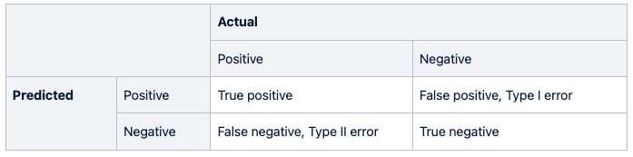
• Precision = positive predictive value = TP / (TP + FP)

• Sensitivity = recall = true positive rate = TP / (TP + FN)

• Specificity = true negative rate = TN / (TN + FP)

• F1 score = \(2 \frac{Precision * Recall}{Precision + Recall}\)

• Matthew’s correlation coefficient = MCC = \(\frac{TP * TN - FP * FN}{\sqrt{(TP+FP)(TP+FN)(TN+FP)(TN+FN)}}\)

  • Between -1 and 1: 1 → perfect prediction, 0 → no better than random, -1 → total disagreement between prediction and observation

6 Confidence Intervals for Machine Learning

See here for more details

• For classification accuracy: assume Gaussian distribution of the proportion, use Binomial proportion confidence interval

  • intervals = z*sqrt( (accuracy * (1-accuracy)) / n)

Nonparametric Confidence Interval

• Use bootstrap resampling:

  • Sample with replacement to get dataset of size n

  • Calculate statistic on sample

  • Repeat (maybe 100 times)

  • Calculate central tendency (median) of 100 sample statistics, and 2.5th and 97.5th percentile

7 Nested Cross Validation

Motivation/Theory, Method/Figure

K-fold cross-validation is used both in the selection of model hyperparameters to configure each model and in the selection of configured model and can lead to overfitting. Each time a model with different model hyperparameters is evaluated on a dataset, it provides information about the dataset.

Method

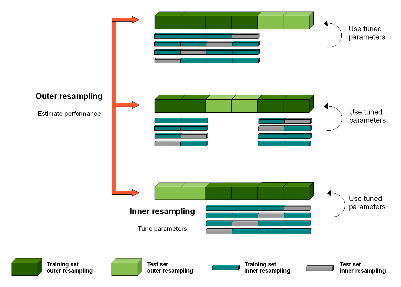
• Split into K fold (outer folds)

• Within each K fold:

  • Split the outer training set (dark green) into L folds (blue/gray)

  • For each L fold:

    • Train each hyperparameter on inner training (blue), test on inner test (gray)

    • For each hyperparameter: average metrics across L folds, choose best

  • Train on outer training (dark green) with best hyperparameter

  • Test on outer test (light green)

• Calculate mean metrics over all K folds

Cost of validation

• Cross-validation = n*k = hyperparameters * models

• Nested cross-validation = L*n*k = inner models * hyperparameters * outer models